Does Increasing TCP Window Size Actually Improve VPN Speeds?

When I updated my GL.iNet article about slow WireGuard connections abroad, I became curious about something I hadn’t actually tested myself: How much of a difference could adjusting TCP receive-window sizes and congestion-control algorithms make to VPN throughput over a high-latency connection?

The theory behind the bandwidth-delay product is well established. Larger TCP windows can help sustain higher throughput over long-distance connections, while congestion-control algorithms such as CUBIC and BBR take different approaches to managing data transmission. But I wanted to see how much these factors actually mattered in practice. Of course, for many digital nomads using employer-managed laptops, changing system-level TCP settings isn’t even an option. Most won’t have the necessary administrative privileges, and modifying those settings on a corporate device generally isn’t advisable anyway. But I was using my personal MacBook Pro in Mexico City, connected through Tailscale to my GL.iNet Flint 2 exit node at home in Virginia. I also had a Linux server in Washington, D.C., that I could use as a controlled TCP sender.

So I decided to experiment. I started by measuring TCP throughput over my Tailscale VPN connection with my Mac’s default automatic receive-buffer limit of approximately 4 MB, comparing CUBIC and BBR using both single and multiple TCP connections. I then increased the buffer limit to approximately 32 MB and repeated the single-connection tests to see whether the larger TCP window would actually improve performance.

What I measured through my home VPN

I ran the test from my MacBook Pro in Mexico City with my home Flint 2 in Virginia selected as my Tailscale exit node. A Linode in Washington, D.C., sent the TCP download to my Mac through the Flint 2’s fiber connection. I verified that my Mac’s public IPv4 address matched my home connection. Tailscale showed a direct connection to the router. Interestingly, my home Flint 2 exit node in Virginia is behind CGNAT, while my client-side connection in Mexico City is not. Despite the home-side CGNAT, Tailscale successfully established a direct peer-to-peer UDP connection, as confirmed by both tailscale status and tailscale ping. This demonstrates that CGNAT doesn't necessarily force Tailscale to use DERP relays. Its NAT traversal mechanisms, including UDP hole punching, can establish direct connectivity depending on the NAT behavior at both endpoints. The Linux TCP sender measured a minimum end-to-end round-trip time of about 110 ms, with readings around 114–115 ms during transfers.

A quick note on why the destination matters. If I connect to the router’s own Tailscale address, the router generates the test data. When I connect to the public address of a server beyond the exit node, the router has to forward that server’s traffic over the tunnel. That second setup is what happens if I were to download a work file through my home connection.

I ran iperf3 in reverse mode so the Linux server sent and the Mac received. Each result below is throughput measured at the Mac over 15 seconds, after a three-second warm-up. The server ran Debian 13 with Linux 6.12 and iperf3 3.18 on one vCPU. My personal Mac ran macOS 27.2.1. This was a sustained TCP download benchmark. It excluded disk writes and file-server application overhead.

What happened when I increased the receiver-buffer maximum?

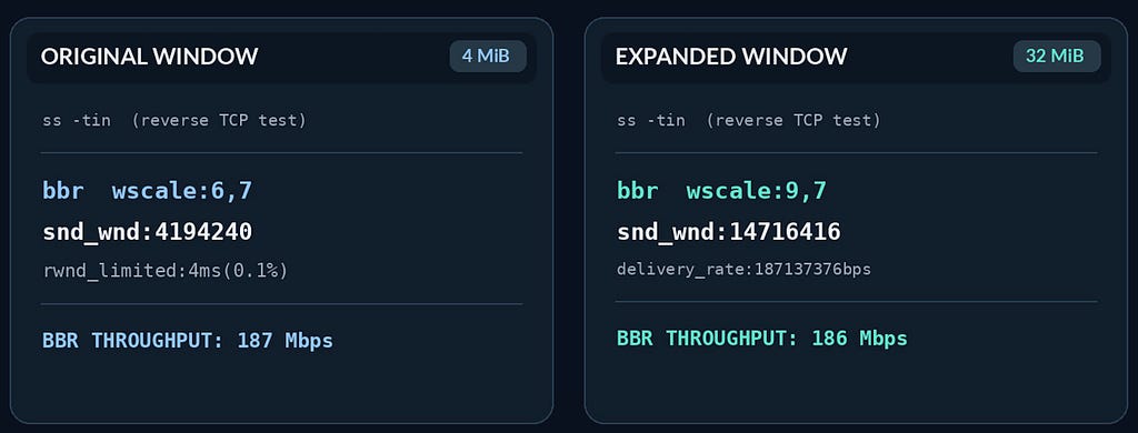
My Mac’s original automatic receive-buffer maximum was 4 MB. Its general socket-buffer ceiling was 8 MB. I temporarily raised both to 32 MB on my personal laptop. I kept the TCP window-scale setting at 3 and used a fresh connection for each run, since TCP establishes window scaling when a connection opens. A MB is 1,048,576 bytes. I use decimal MB for the bandwidth calculations below.

To find out what happened on the wire, I inspected the Linux sender’s TCP socket. Its snd_wnd field reports the receive window the Mac advertised. In the original BBR run I saw 4,194,240 bytes, just 64 bytes shy of 4 MB. In the expanded run I saw 14,716,416 bytes. The Mac’s negotiated window-scale shift rose from 6 to 9, even though its scale setting still read 3. Apple’s published TCP code can select a higher shift to accommodate a larger receive buffer.

One download, two congestion-control algorithms

While the Mac advertises how much data it’s prepared to receive through its TCP receive window, the sender has its own mechanism for controlling how much unacknowledged data it can have in flight: TCP congestion control.

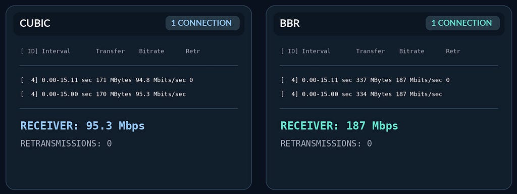
Two algorithms worth comparing are CUBIC and BBR. CUBIC is a loss-based algorithm that adjusts its congestion window in response to network congestion, while BBR takes a different approach, estimating bottleneck bandwidth and round-trip propagation time to determine its sending behavior. An important distinction is that TCP congestion control operates at the sending endpoint. When downloading a file, the remote server controls the congestion-control algorithm, while your laptop controls the advertised receive window. For uploads, the roles are reversed, and your laptop’s congestion-control algorithm becomes relevant. This also means changing the TCP congestion-control algorithm on a travel router or VPN exit node won’t affect TCP connections the router simply forwards. Since I controlled both endpoints in this experiment, I could independently adjust the receive-buffer settings on my Mac and switch between CUBIC and BBR on the Linux server generating the download traffic. This allowed me to compare how each algorithm performed over the same VPN connection.

One detail from the slower 89.9 Mbps CUBIC run helps explain why increasing the receive window didn’t improve performance. Near the end of that test, the Mac was advertising a receive window of 12.46 MB, but the server’s congestion window was only 920 segments of 1,228 bytes, or approximately 1.13 MB. At the measured 114 ms RTT, that congestion-window size corresponds to a theoretical throughput of roughly 79 Mbps. The Mac received 77.9 Mbps during the final second, remarkably close to that calculation.

In other words, the sender’s congestion window was much smaller than the receive window my Mac was advertising. Increasing the receiver’s window further wasn’t going to help while the sender was already constrained by its own congestion control.

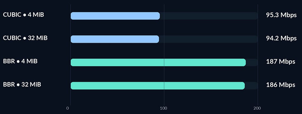
BBR delivered roughly twice CUBIC’s single-connection throughput in this session. These were short, sequential tests on one internet path. I did not alternate the algorithms across repeated trials or measure CPU saturation on the single-vCPU server and the exit node.

Four TCP connections speed-test

With the Mac at its original settings, I repeated the download using four independent TCP connections at once.

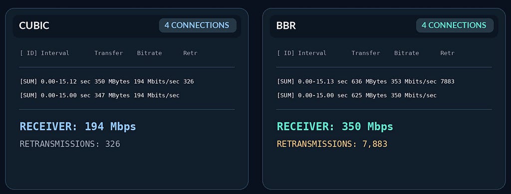
This is how a speed test and a file download can give you different answers from the same desk. Under BBR, my Mac received 350 Mbps across four connections while one connection delivered 187 Mbps. Even the faster result came with considerably more retransmissions. I ran the four-connection comparison at the original buffer settings only.

For remote work, the distinction is whether your application can split the work across independent transport connections. A single SFTP transfer commonly uses one SSH connection. A browser can fetch many resources at once over HTTP/2 while sharing one TCP connection. HTTP/3 uses QUIC over UDP and has its own flow control. Counting downloads or browser tabs alone won’t tell you which case you’re in. So when would 4 MB actually cost me speed?

Take a traveler with symmetric gigabit service at both ends. To sustain a given rate on one TCP connection, multiply the rate in bits per second by the end-to-end RTT in seconds, then divide by eight to get bytes in flight.

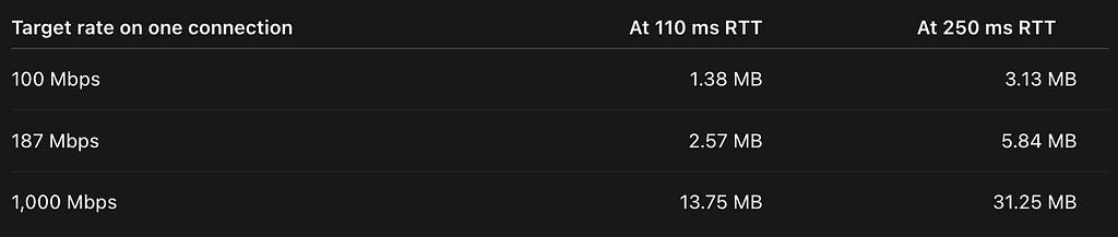
At my measured RTT, the original 4 MB window could theoretically support about 305 Mbps on one connection. My 187 Mbps download needed about 2.57 MB in flight. In one original BBR socket sample, the sender had spent only 4 milliseconds out of 4.76 busy seconds limited by the receive window. That helps explain why the larger window bought me so little.

Now take that same 187 Mbps download to a 250 ms path. It would need 5.84 MB in flight. If the receiver could advertise only 4 MB, the one-connection ceiling would fall to about 134 Mbps. That’s where I’d go looking for a window limit. A call or an email exchange has much less data to move. These tests show that my Mac could advertise its full original window during a sustained download. They can’t tell us how often a typical laptop does so. So while gigabit speeds at both ends make the question worth asking, you still don’t know how much bandwidth the route between them can deliver.

It’s also worth considering that my tests were conducted between Mexico City and Virginia, with approximately 110 ms RTT. Someone connecting from Southeast Asia to a home VPN server in the United States could experience substantially higher latency, along with inefficient ISP peering, congested international routes, or packet loss. In those situations, the network path itself may limit throughput well before TCP receive-window sizing becomes relevant. At the same time, higher RTT increases the amount of data needed in flight to sustain high speeds, making TCP window sizing potentially more important. Which factor matters most depends on the actual connection.

Windows offers a useful comparison. Microsoft documents a shift of 8 for the Normal autotuning example on Windows Server. A TCP connection using that shift can represent up to 16,776,960 bytes, or about 537 Mbps at 250 ms on one connection. I didn’t benchmark Windows simply because I don’t own a Windows machine. On a particular work laptop though, the negotiated shift and the window advertised during the download are the two numbers I’d want.

Is ESnet’s Warning About Wi-Fi Still Relevant?

ESnet’s macOS tuning guide is where I found the 32 MB buffer recommendation. Interestingly, the guide also advises against applying these settings to laptops primarily connected over Wi-Fi. I think that warning deserves some qualification given the capabilities of modern wireless networking. Wi-Fi 6E and Wi-Fi 7 can deliver gigabit and even multigigabit throughput under suitable conditions. In a Wireless Broadband Alliance enterprise trial, a Wi-Fi 7 client sustained over 1 Gbps up to 40 feet from the access point using a 160 MHz channel at 6 GHz. In conversations with Ken from RemoteToHome, I also confirmed he has been able to achieve 2.5+ Gbps on Wi-Fi 7 MLO (STR-MLMR) using GL.iNet routers in his own tests.

Of course, Wi-Fi performance varies considerably with signal strength, interference, and network congestion, so increasing TCP buffers isn’t automatically beneficial. But the fact that a laptop connects over Wi-Fi shouldn’t, by itself, rule out TCP receive-window limitations on a high-bandwidth connection.

Conclusion

For digital nomads using managed work laptops, changing TCP settings usually isn’t practical anyway. But you can still learn a lot by comparing single-connection and multi-connection speeds through your home VPN. If several connections are significantly faster than one, it suggests your VPN has more total capacity than an individual transfer is taking advantage of. That doesn’t tell you exactly what’s causing the difference, but it’s a useful starting point.

My own experiment demonstrated why simply increasing TCP window sizes isn’t always the answer. I increased my Mac’s automatic receive-buffer maximum from 4 MiB to 32 MiB and confirmed that it could advertise a much larger receive window. Yet my download speeds barely changed. The Mac was already capable of accepting data faster than the server was delivering it.

What made a much bigger difference in my tests was changing the server’s TCP congestion-control algorithm from CUBIC to BBR, which nearly doubled single-connection throughput.

So, just because you have gigabit internet at both ends of your VPN doesn’t mean every download will achieve gigabit speeds. A larger TCP window can help when it’s actually the bottleneck, but it won’t magically make a slow connection faster when something else is holding it back.